In all Machine Learning algorithms, linear regression happened to be the most straightforward and easy to understand as it uses the straight line’s formula, which we have learned in the high school mathematics course. But at the beginning of the machine learning course, we start by using the sci-kit learn library, and then our true understanding of linear regression got a halt. Thus, many of us didn’t truly understand this easy to implement and easy to use algorithm. Here I’ll present a simple and intuitive way of implementing the linear regression line from scratch.
At first, I have used a function that will take the data from the user. In reality, we will get our data from different sources like Kaggle or from other different sources as a CSV file. But to get a real understanding, we will give our own data.
After that, I have presented two implementation methods; the first one is by the iteration method, where we will find the minimum value of the loss function. This process is called the Gradient Descent algorithm.
In ML, cost functions are used to estimate how badly models are performing. Put simply, a cost function is a measure of how wrong the model is in terms of its ability to estimate the relationship between X and y. This is typically expressed as a difference or distance between the predicted value and the actual value.
https://towardsdatascience.com
In simple terms, the cost or loss function is nothing but a mathematical expression where it shows the difference between the predicted values and the actual values over the length of the data.
We will use the Mean Squared Error function to calculate the loss/cost. There are few steps; find the difference between predicted and actual values, square the difference and finally find the mean of the squares for every value.
This is a very bright idea to use the difference’s square instead of only using the difference between the predicted and actual values. Due to square operation, the function will be minimized only when the values are close to each other. If the two values are equal, then the cost function will be zero, which we want to obtain.
\begin{aligned}
 MSE = \frac{1}{n} \sum_{i=0}^{n} (y_i - \bar y_i)^2
\end {aligned}
yi = actual value and yˉi = predicted value
\begin{aligned}
 MSE = \frac{1}{n} \sum_{i=0}^{n} (y_i - (mx_i + c))^2
\end {aligned} yˉi is substituted by (mxi+c )
Now that we have defined the loss function and understood, the lower the loss function, the better the model. But how would we know which is the lowest value of the loss/cost function? Fortunately, Geoffrey Hinton came up with the idea of using the Gradient Descent into Machine Learning. It is an algorithm for searching for the lowest point ( >=0 ) in the cost function. We will use this Gradient Descent algorithm and find the minimum point of the proposed cost function.
By calculating the partial derivative of the cost/loss function w.r.t m and c we get the Dm and Dc which is supposed to be zero in the iteration. As we know derivative of a function is zero means the function value is almost constant around that value, and the update of the m and c will be slow at that point of time.
D_{m} = \frac{-2}{n} \sum_{i=0}^{n} (x_i(y_i - \bar y_i)
D_{c} = \frac{-2}{n} \sum_{i=0}^{n} (y_i - \bar y_i)
At the beginning, the value of m and c is given as 0. Then we have to set learning rate L and iteration number, epoch. This for loop runs for the given number of times assigned in the epoch. So after a given number of iteration, we will get a value of m and c.
m = m-L \ × \ D_m\\ c = c \ -\ L \ × D_c
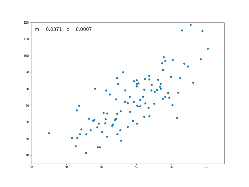
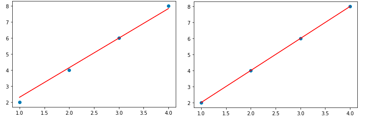
In the next section, we just made a regression line Y_pred and plotted the line.